Aboveground biomass in LTFEM plots
Data
Data from WYK plots are from surveys in 2022.
Data from NSSF plots are from surveys in 2020.
Data from NatureParks and Mandai plots are from surveys in 2023.
Height-DBH models
plotSets <- c("WYK", "NatureParks", "NSSF")
mods_HD <- lapply(plotSets, function(s) {
    list(nls_LL = nls(height_avg ~ a*DBH^b, data = treeHeights[[s]], start = list(a=exp(1), b = 0.5)),
         nls_WB = nls(height_avg ~ a*(1-exp(-b*DBH^c)), data = treeHeights[[s]], start = list(a=44,b=0.05,c=0.8)),
         nls_MM = nls(height_avg ~ (a*DBH)/(b + DBH), data = treeHeights[[s]], start = list(a=48, b = 38)))
})
names(mods_HD) <- plotSets

mods_HD_aictab <- lapply(mods_HD, function(m) {
    AICcmodavg::aictab(m)
})

DBH_minmax <- lapply(treeHeights, function(df) range(df$DBH, na.rm = TRUE))
WYK plots:
mods_HD_aictab$WYK %>%
  data.frame(row.names = NULL) %>%
  select(-c(AICc, Cum.Wt, LL)) %>%
  rename(Model = Modnames,
         k = K,
         "Δ AICc" = Delta_AICc,
         L = ModelLik,
w = AICcWt)| Model | k | Δ AICc | L | w |
|---|---|---|---|---|
| nls_WB | 4 | 0.000000 | 1.0000000 | 0.5135824 |
| nls_LL | 3 | 1.417049 | 0.4923701 | 0.2528726 |
| nls_MM | 3 | 1.576072 | 0.4547370 | 0.2335449 |
Nature Parks:
mods_HD_aictab$NatureParks %>%
  data.frame(row.names = NULL) %>%
  select(-c(AICc, Cum.Wt, LL)) %>%
  rename(Model = Modnames,
         k = K,
         "Δ AICc" = Delta_AICc,
         L = ModelLik,
w = AICcWt)| Model | k | Δ AICc | L | w |
|---|---|---|---|---|
| nls_MM | 3 | 0.0000000 | 1.0000000 | 0.4249602 |
| nls_LL | 3 | 0.2032201 | 0.9033817 | 0.3839012 |
| nls_WB | 4 | 1.5979933 | 0.4497800 | 0.1911386 |
Nee Soon:
mods_HD_aictab$NSSF %>%
  data.frame(row.names = NULL) %>%
  select(-c(AICc, Cum.Wt, LL)) %>%
  rename(Model = Modnames,
         k = K,
         "Δ AICc" = Delta_AICc,
         L = ModelLik,
w = AICcWt)| Model | k | Δ AICc | L | w |
|---|---|---|---|---|
| nls_WB | 4 | 0.0000000 | 1.0000000 | 0.4029002 |
| nls_MM | 3 | 0.0700559 | 0.9655784 | 0.3890318 |
| nls_LL | 3 | 1.3216475 | 0.5164257 | 0.2080680 |
Power (or ‘log-log’) model
\(H = a D^b\)
(which can be linearised to \(\log H = a' + b \log D\) where \(a' = \log a\))
where H is the height of the tree in metres and D is the diameter at the point of measurement in cm.
sapply(mods_HD, function(m) {
    m$nls_LL$m$getPars()
}) %>%
    t() %>%
    data.frame() %>%
rownames_to_column(var = "Plot set")| Plot set | a | b |
|---|---|---|
| WYK | 3.445676 | 0.5243473 |
| NatureParks | 2.463684 | 0.5769609 |
| NSSF | 3.567342 | 0.4997321 |
mods_HD_pred_LL <- lapply(plotSets, function(s) {
    D_new <- seq(DBH_minmax[[s]][1],
                 DBH_minmax[[s]][2],
                 length.out = 1000)

    data.frame(D = D_new,
               fit = predict(mods_HD[[s]]$nls_LL,
                        newdata = data.frame(DBH = D_new)))
})
names(mods_HD_pred_LL) <- plotSets

ggplot() +
    theme_classic() +
    geom_point(data = treeHeights$WYK,
               mapping = aes(x = DBH, y = height_avg),
               color = "darkgreen") +
    geom_line(data = mods_HD_pred_LL[["WYK"]],
              mapping = aes(x = D, y = fit),
              color = "darkgreen") +
    geom_point(data = treeHeights$NatureParks,
               mapping = aes(x = DBH, y = height_avg),
               color = "red") +
    geom_line(data = mods_HD_pred_LL[["NatureParks"]],
              mapping = aes(x = D, y = fit),
              color = "red") +
    geom_point(data = treeHeights$NSSF,
               mapping = aes(x = DBH, y = height_avg),
               color = "blue") +
    geom_line(data = mods_HD_pred_LL[["NSSF"]],
              mapping = aes(x = D, y = fit),
              color = "blue") +
    scale_y_continuous(trans = "log10") +
    scale_x_continuous(trans = "log10") +
    labs(x = "DBH (cm)", y = "Height (m)")
Weilbull
Not used for calculations here but fitted for information.
\(H = \alpha (1 - e^{-(D/\beta)^\gamma})\)
where H is the height of the tree in metres and D is the diameter at the point of measurement in cm.
sapply(mods_HD, function(m) {
    m$nls_WB$m$getPars()
}) %>%
    t() %>%
    data.frame() %>%
    rownames_to_column(var = "Plot set") %>%
    rename(`$\\alpha$` = "a",
           "$\\beta$" = "b",
           "$\\gamma$" = "c") %>%
knitr::kable()| Plot set | \(\alpha\) | \(\beta\) | \(\gamma\) |
|---|---|---|---|
| WYK | 43.90884 | 0.0585514 | 0.7061825 |
| NatureParks | 41.55518 | 0.0446820 | 0.7450690 |
| NSSF | 47.47136 | 0.0447680 | 0.7333806 |
mods_HD_pred_WB <- lapply(plotSets, function(s) {
    D_new <- seq(DBH_minmax[[s]][1],
                 DBH_minmax[[s]][2],
                 length.out = 1000)

    data.frame(D = D_new,
               fit = predict(mods_HD[[s]]$nls_WB,
                        newdata = data.frame(DBH = D_new)))
})
names(mods_HD_pred_WB) <- plotSets

ggplot() +
    theme_classic() +
    geom_point(data = treeHeights$WYK,
               mapping = aes(x = DBH, y = height_avg),
               color = "darkgreen") +
    geom_line(data = mods_HD_pred_WB[["WYK"]],
              mapping = aes(x = D, y = fit),
              color = "darkgreen") +
    geom_point(data = treeHeights$NatureParks,
               mapping = aes(x = DBH, y = height_avg),
               color = "red") +
    geom_line(data = mods_HD_pred_WB[["NatureParks"]],
              mapping = aes(x = D, y = fit),
              color = "red") +
    geom_point(data = treeHeights$NSSF,
               mapping = aes(x = DBH, y = height_avg),
               color = "blue") +
    geom_line(data = mods_HD_pred_WB[["NSSF"]],
              mapping = aes(x = D, y = fit),
              color = "blue") +
    scale_y_continuous(trans = "log10") +
    scale_x_continuous(trans = "log10") +
    labs(x = "DBH (cm)", y = "Height (m)")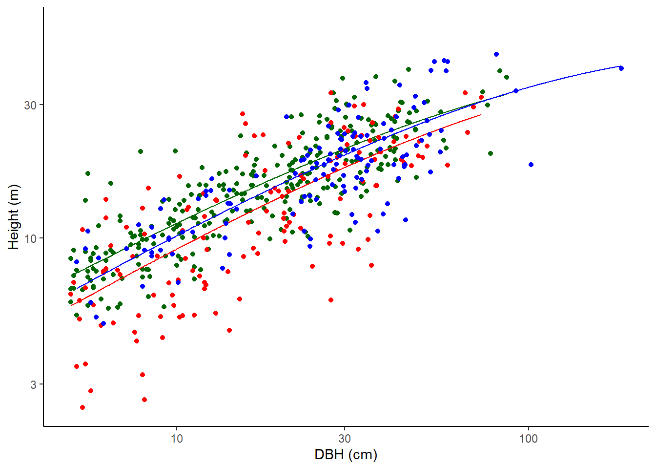
Michaelis-Menten
Not used for calculations here but fitted for information.
\(H = (A \times D)/(B + D)\)
where H is the height of the tree in metres and D is the diameter at the point of measurement in cm.
sapply(mods_HD, function(m) {
    m$nls_MM$m$getPars()
}) %>%
    t() %>%
    data.frame() %>%
    rownames_to_column(var = "Plot set") %>%
rename(A = a, B = b)| Plot set | A | B |
|---|---|---|
| WYK | 39.45488 | 25.65579 |
| NatureParks | 37.91217 | 32.36861 |
| NSSF | 47.04560 | 40.06679 |
mods_HD_pred_MM <- lapply(plotSets, function(s) {
    D_new <- seq(DBH_minmax[[s]][1],
                 DBH_minmax[[s]][2],
                 length.out = 1000)

    data.frame(D = D_new,
               fit = predict(mods_HD[[s]]$nls_MM,
                        newdata = data.frame(DBH = D_new)))
})
names(mods_HD_pred_MM) <- plotSets

ggplot() +
    theme_classic() +
    geom_point(data = treeHeights$WYK,
               mapping = aes(x = DBH, y = height_avg),
               color = "darkgreen") +
    geom_line(data = mods_HD_pred_MM[["WYK"]],
              mapping = aes(x = D, y = fit),
              color = "darkgreen") +
    geom_point(data = treeHeights$NatureParks,
               mapping = aes(x = DBH, y = height_avg),
               color = "red") +
    geom_line(data = mods_HD_pred_MM[["NatureParks"]],
              mapping = aes(x = D, y = fit),
              color = "red") +
    geom_point(data = treeHeights$NSSF,
               mapping = aes(x = DBH, y = height_avg),
               color = "blue") +
    geom_line(data = mods_HD_pred_MM[["NSSF"]],
              mapping = aes(x = D, y = fit),
              color = "blue") +
    scale_y_continuous(trans = "log10") +
    scale_x_continuous(trans = "log10") +
    labs(x = "DBH (cm)", y = "Height (m)")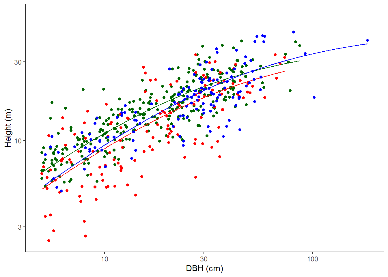
Calculate aboveground biomass
## Warning in par(oldpar): calling par(new=TRUE) with no plot
## Warning in par(oldpar): calling par(new=TRUE) with no plot
## The reference dataset contains 16467 wood density values## Your taxonomic table contains 568 taxa## The reference dataset contains 16467 wood density values## Your taxonomic table contains 269 taxaknitr::kable(plots_AGBsum, "html") %>%
kableExtra::kable_styling("striped") %>%
kableExtra::scroll_box(height = "500px", width = "100%")| plotID | trees | bigTrees | plotSet |
|---|---|---|---|
| AQ1 | 168.76308 | 56.524670 | Mandai |
| AQ2 | 114.28906 | 25.882724 | Mandai |
| AQ3 | 138.68224 | 76.103103 | Mandai |
| AQ4 | 222.01711 | 55.287869 | Mandai |
| AQ5 | 108.77621 | NA | Mandai |
| AQ6 | 261.53009 | 176.039038 | Mandai |
| AQ7 | 118.75840 | 79.754197 | Mandai |
| BBN1 | 123.81603 | 136.893086 | NatureParks |
| BBN2 | 128.20371 | 213.949394 | NatureParks |
| BBN3 | 870.04069 | 419.032141 | NatureParks |
| BBN4 | 310.92692 | 123.429420 | NatureParks |
| BBN5 | 106.50115 | 72.322744 | NatureParks |
| BBT1 | 148.40721 | 143.401934 | NatureParks |
| BBT2 | 143.88328 | 131.373639 | NatureParks |
| BBT3 | 270.71848 | 77.993642 | NatureParks |
| BBT4 | 113.13407 | 92.375619 | NatureParks |
| BBT5 | 243.22769 | 124.542606 | NatureParks |
| GA1 | 201.43357 | 106.369569 | NatureParks |
| GA2 | 160.03259 | 67.844372 | NatureParks |
| GA3 | 202.20431 | 189.818971 | NatureParks |
| GA4 | 144.34307 | 53.373039 | NatureParks |
| GA5 | 162.80153 | 64.327095 | NatureParks |
| HQ1 | 108.08933 | 89.300979 | Mandai |
| Q1 | 197.34085 | 46.919991 | NSSF |
| Q10 | 113.03175 | 27.592775 | NSSF |
| Q101 | 171.07465 | 39.043477 | NSSF |
| Q102 | 31.21174 | 242.527247 | NSSF |
| Q104 | 224.02435 | 41.386066 | NSSF |
| Q105 | 158.57057 | 51.052289 | NSSF |
| Q107 | 146.75948 | 95.193229 | NSSF |
| Q109 | 202.22742 | 76.233718 | NSSF |
| Q111 | 94.81840 | 13.855673 | NSSF |
| Q112 | 1391.83781 | 621.642245 | NSSF |
| Q2 | 84.42926 | 45.279447 | NSSF |
| Q203a | 173.52439 | 180.194587 | NSSF |
| Q206 | 113.94121 | 62.708773 | NSSF |
| Q208 | 188.32439 | 52.735904 | NSSF |
| Q209 | 141.73692 | 8.804949 | NSSF |
| Q213 | 138.54019 | 63.812413 | NSSF |
| Q217 | 139.50190 | 47.215561 | NSSF |
| Q220 | 116.73491 | 43.488430 | NSSF |
| Q3 | 241.02072 | 104.810999 | NSSF |
| Q301 | 114.99704 | 82.642628 | NSSF |
| Q302 | 165.70699 | 78.788742 | NSSF |
| Q305 | 90.05246 | 57.773743 | NSSF |
| Q306 | 95.67252 | 77.285461 | NSSF |
| Q307 | 86.50610 | 60.430823 | NSSF |
| Q308a | 153.35999 | 75.951804 | NSSF |
| Q311a | 59.87842 | 39.901935 | NSSF |
| Q319a | 141.02891 | 34.516390 | NSSF |
| Q320a | 66.97533 | 26.594493 | NSSF |
| Q4 | 170.31269 | 83.582254 | NSSF |
| Q404a | 260.24193 | 70.194890 | NSSF |
| Q405 | 97.34242 | 33.430648 | NSSF |
| Q408 | 97.13591 | 68.569353 | NSSF |
| Q414a | 174.69147 | 41.987289 | NSSF |
| Q504 | 156.42538 | 66.916645 | NSSF |
| Q509 | 799.85922 | 345.477473 | NSSF |
| Q6 | 440.62235 | 147.100137 | NSSF |
| Q7 | 97.13678 | 49.152938 | NSSF |
| Q8 | 226.75107 | 109.749620 | NSSF |
| Q9 | 308.42778 | 97.904593 | NSSF |
| UT1 | 141.46932 | 78.946414 | NatureParks |
| UT2 | 136.99899 | 60.011894 | NatureParks |
| UT3 | 312.21579 | 211.535213 | NatureParks |
| UT4 | 130.02602 | 150.911333 | NatureParks |
| UT5 | 243.30202 | 186.669671 | NatureParks |
| W01 | 156.09023 | 83.742488 | WYK |
| W02 | 146.70648 | 35.007526 | WYK |
| W03 | 124.30847 | 69.073569 | WYK |
| W04 | 329.63424 | 187.848491 | WYK |
| W05 | 123.93502 | 44.911719 | WYK |
| W06 | 822.24643 | 433.164001 | WYK |
| W07 | 291.84092 | 290.831693 | WYK |
| W08 | 126.88531 | 137.929828 | WYK |
| W09 | 194.82655 | 65.179803 | WYK |
| W10 | 276.71959 | 93.269864 | WYK |
| W11 | 94.12767 | 271.316579 | WYK |
| W12 | 209.60280 | 123.901134 | WYK |
| W13 | 437.75780 | 169.043591 | WYK |
| W14 | 12.96328 | 31.627540 | WYK |
| W15 | 386.80608 | 215.467525 | WYK |
| W16 | 122.85741 | 144.957804 | WYK |
| W17 | 161.73570 | 181.580314 | WYK |
| W18 | 162.09229 | 43.118042 | WYK |
| W19 | 288.13384 | 235.342462 | WYK |
| W20 | 126.82501 | 74.260173 | WYK |
| W21 | 153.78698 | 172.987710 | WYK |
| W22 | 151.00536 | 215.817836 | WYK |
| W23 | 159.47115 | 54.131284 | WYK |
| W24 | 186.40299 | 137.839350 | WYK |
| W25 | 197.58309 | 49.003036 | WYK |
| W26 | 187.60133 | 92.598254 | WYK |
| W27 | 255.36176 | 119.550588 | WYK |
| W28 | 190.90326 | 105.874147 | WYK |
| W29 | 308.64480 | 383.546263 | WYK |
| W30 | 197.58065 | 133.736939 | WYK |
| W31 | 198.55310 | 108.400565 | WYK |
| W32 | 118.43561 | 76.694902 | WYK |
| W33 | 246.44698 | 123.873324 | WYK |
| W34 | 122.52789 | 121.282885 | WYK |
| W35 | 67.72131 | 45.775982 | WYK |
| W36 | 168.41002 | 122.547187 | WYK |
| W37 | 79.66613 | 29.398764 | WYK |
| W38 | 147.97113 | 125.596976 | WYK |
| W39 | 109.77155 | 44.694969 | WYK |
| W40 | 159.81659 | 47.042167 | WYK |
| W41 | 181.17761 | 65.077784 | WYK |
| W42 | 210.78335 | 89.448103 | WYK |
| W44 | 204.10663 | 131.737592 | WYK |
| W45 | 162.86635 | 23.617308 | WYK |
| W46 | 122.73458 | 33.908155 | WYK |
| W47 | 81.81173 | 57.555797 | WYK |
| W48 | 262.31518 | 93.820620 | WYK |
| W49 | 569.15859 | 176.131470 | WYK |
| W50 | 113.27596 | 63.909157 | WYK |
| W51 | 315.96524 | 124.172082 | WYK |
| W52 | 141.90954 | 83.699864 | WYK |
| W53 | 230.64573 | 141.159493 | WYK |
| W54 | 242.93373 | 79.534635 | WYK |
| W55 | 181.23666 | 190.309757 | WYK |
| W56 | 128.16780 | 32.886871 | WYK |
| W57 | 112.75134 | 54.548686 | WYK |
| W58 | 330.59702 | 177.027683 | WYK |
| W59 | 76.25737 | 58.099651 | WYK |
| W60 | 301.72293 | 155.161842 | WYK |
| W62 | 287.18051 | 84.170950 | WYK |
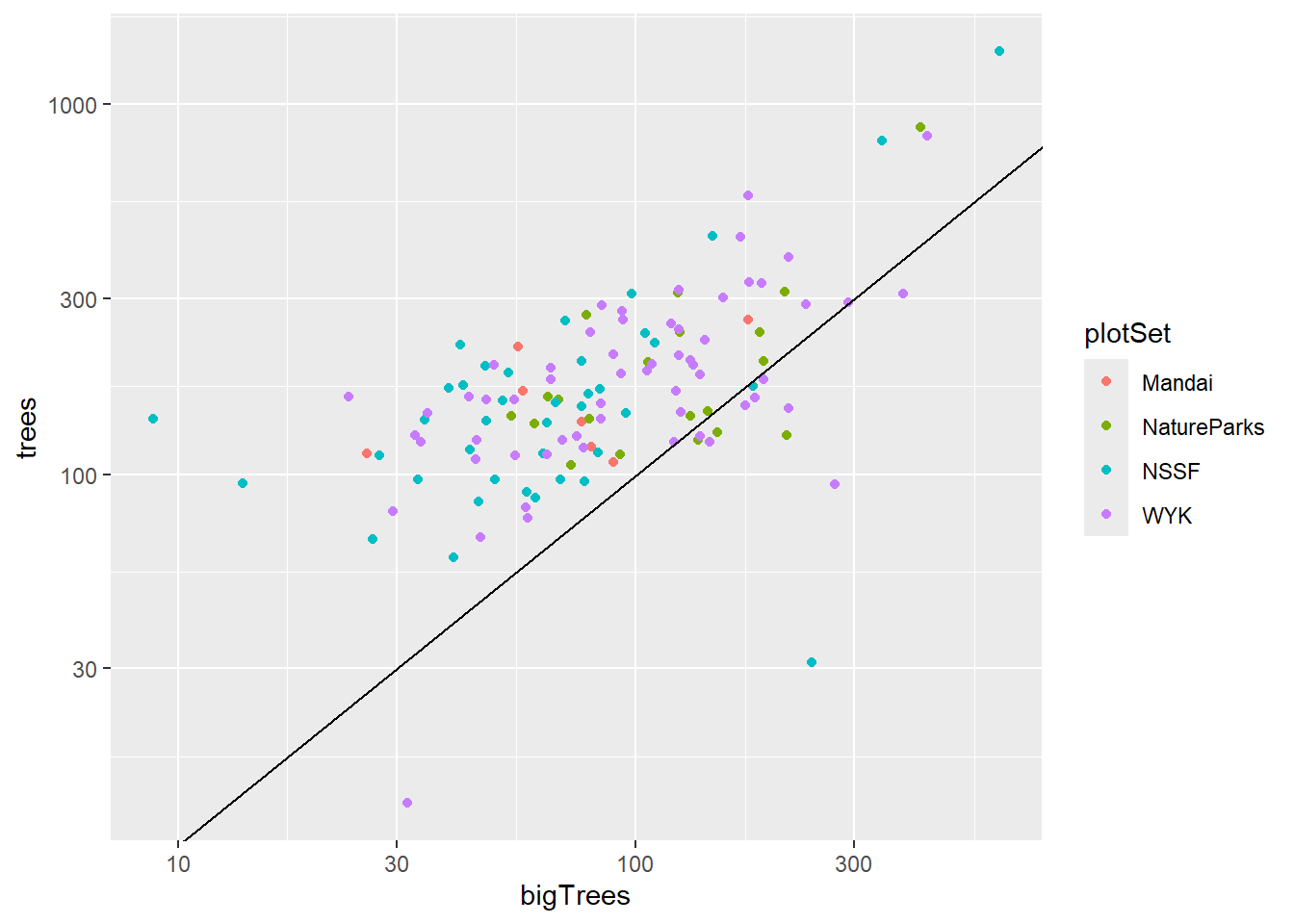
Note: there were no big trees in AQ5.
ggplot(data = plots_AGBsum) +
    geom_point(mapping = aes(y = trees, x = bigTrees, col = plotSet)) +
    scale_y_continuous(trans = "log10") +
    scale_x_continuous(trans = "log10") +
    geom_abline(intercept = 0, slope = 1)